Schottky fractals

The magic begins when we configure two or more nonoverlapping sets of paired disks in the complex plane. Under repeated mappings, disks proliferate into beautiful fractal forms. Such an arrangement of disks and transformations is known as Schottky dynamics in honor of Frederich Schottky who explored the underlying mathematics in the late 1800s.¹

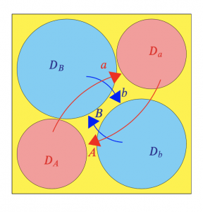
Here we work with two sets of paired disks: The disks $D_A$ and $D_a$ are paired by the transformation $a$ , and the disks $D_B$ and $D_b$ are paired by the transformation $b$ . These are depicted in the following figure.²

In the following program, the two transformations $a$ and $b$ and their inverses, $A=a^{-1}$ and $B=b^{-1}$ , are iteratively applied to the four seed disks up to nbrLevels many levels.

Schottky fractals

Here’s one way to understand what’s going on. Set nbrLevels to 0, model to ‘disks’, and color model to ‘by disk’. This assigns a random color to each of the four seed disks. Keep pressing the Randomize button until these four colors are quite distinct. Next set nbrLevels to 1, and let’s call any one of the seed disks $D_a$ . Because the disks $D_A$ and $D_a$ are paired, the transformation $a$ maps the outside of $D_A$ to the inside of $D_a$ . There are three seed disks that lie outside $D_A$ : $D_b$ , $D_B$ , and $D_a$ . Applying $a$ to each of these produces a new disk of the same color inside $D_a$ . Increase nbrLevels from 1 to 2 and the process repeats. Each level 1 disk residing inside $D_a$ maps three seed disks to even smaller disks in its interior. Since $D_a$ was chosen arbitrarily, the same process occurs in each of the seed disks.

Let’s look a bit more closely. Every disk represents a composition of the four transformations $a$ , $A$ , $b$ , and $B$ . This is indicated by the subscript in the disk’s name. For example, the seed disk $D_a$ represents the transformation $a$ . Apply $a$ to seed disk $D_b$ and we get the (smaller) disk $D_{ab}$ contained in $D_a$ . In turn, disk $D_{ab}$ represents the transformation $ab$ . Applying $ab$ to the seed disk $D_A$ yields a new (even smaller) disk $D_{abA}$ nested inside $D_{ab}$ . In general, applying the composite transformation $T$ to three seed disks yields three smaller disks nesting inside disk $D_T$ . And why do we apply $T$ to three rather than to all four seed disks? Consider, for example, the disk $D_{ab}$ . If we were to apply this to the seed disk $D_B$ we obtain $D_{abB}$ . But since $b$ and $B$ are inverses, $D_{abB}$ is another name for $D_a$ , and our goal is to produce lower-level nested disks, not to backtrack. So the three disks nested in $D_{ab}$ one level lower are $D_{abA}$ , $D_{aba}$ , and $D_{abb}$ .³D_b[/latex], $D_a$ , and $D_A$ the noncancelling seed disks of $D_b$ .]

When model is set to ‘disks’, the disks at every level are rendered. When model is ‘spheres’, disks are represented by spheres, but only those spheres at level nbrLevels get rendered.

As we’ve seen, setting color model to ‘by disk’ assigns a color to each of the four seed disks and propagates these colors to higher levels: a disk’s color is that of the seed disk from which it was transformed. Setting color model to ‘by level’ assigns a random color to each level.

Prev Next

See Indra’s Pearls, Chapter 4. ↩
Indra’s Pearls, Chapter 4, Figure 4.1. ↩
We call [latex ↩

Michael Laszlo

It is not a something, but not a nothing either

Schottky fractals